УДК 519.6:519.725:681.3
(ВВЕДЕНИЕ В ВЕЙВЛЕТЫ
И ВЕЙВЛЕТ-ПРЕОБРАЗОВАНИЯ)
©1998 г. Max Fomitchev
Вейвлеты - это математические функции, позволяющие анализировать различные частотные компоненты данных. Вейвлеты обладают существенными преимуществами по сравнению с преобразованием Фурье, потому что с их помощью можно легко анализировать прерывистые сигналы, либо сигналы с острыми всплесками. Кроме того вейвлеты позволяют анализировать данные согласно масштабу, на одном из заданных уровней (мелком или крупном). Эффективная реализация вейвлет-преобразование (пирамидальный алгоритм) позволяет выполнять анализ данных за время порядка O(N). Уникальные свойства вейвлетов позволяют сконструировать базис, в котором представление данных будет выражаться всего несколькими ненулевыми коэффициентами. Это свойство делает вейвлеты очень привлекательными для упаковки данных, в том числе видео- и аудио-информации. Мелкие коэффициенты разложения могут быть отброшены в соответствии с выбранным алгоритмом без значительного влияния на качество упакованных данных. Вейвлеты нашли широкое применение в цифровой обработке изображения, обработке сигналов и анализе данных.
Эта статья является кратким
введением в теорию вейвлетов. Описаны прямое и
обратное вейвлет-преобразования и основные
области применения вейвлетов (компрессия
подвижного и неподвижного изображения,
фильтрация шума, генерация музыкальных тонов и
реконструкция ультразвукового изображения).
Wavelets are mathematical functions that decompose data into different frequency components. Wavelets analyze each frequency component with resolution corresponding to its scale. Wavelets have advantages over Fourier transform in analyzing signals with discontinuities and sharp spikes. Wavelet transform can be done efficiently in O(N) time. Due to its unique properties appropriately chosen wavelet basis requires few non-zero wavelet coefficients to represent data functions. This property makes wavelets ideal for data compression. Also, small wavelet coefficients can be discarded (thresholding) without substantially affecting reconstructed data. Wavelets are intensively used in digital image processing, signal compression and data analysis.
This paper is a brief introduction to wavelet theory. It explains forward and inverse wavelet transform and most common wavelet applications (still and motion image compression, noise filtering, music tones generation and ultrasound imaging).
Key words: wavelets, wavelet transform, image compression.
1. Introduction
2. Wavelets
2.1. Review of the mathematics
2.2. Examples of wavelets
2.3. Wavelet data representation
3. Wavelet transforms
3.1. Discreet wavelet transform
3.2. Mallat's pyramidal algorithm
3.3. Pyramid algorithm implementation
3.4. Thresholding
4. Wavelet applications
4.1. Still image compression
4.2. Video sequence compression
4.3. Artificial vision
4.4. Noise filtering
4.5. Musical tones synthesis
4.6. Detecting quasi-periodic oscillations
4.7. Ultrasound imaging
5. Conclusion
1. Introduction
The fundamental idea behind wavelets is to analyze according to scale.
Wavelets are functions that satisfy certain mathematical requirements and are used in representing data or other functions. In wavelet analysis the scale that we use to look at data plays a special role. Wavelet algorithms process data at different scales or resolutions, emphasizing data's gross or small features.
Scientists have always wanted more appropriate functions than sines and cosines which comprise the basis of Fourier analysis, to approximate signals with discontinuities. Sines and cosines are non-local and stretch out to infinity. Therefore they do a very poor job in approximating signals with sharp spikes. But with wavelet analysis, we can use approximating functions that are contained in finite domains.
The wavelet analysis procedure employs a wavelet prototype function, called mother wavelet. Temporal analysis is performed with a contracted high frequency version of mother-wavelet, while frequency analysis is performed with a dilated, low frequency version of the same wavelet. Because the original signal or function can be represented in terms of a wavelet expansion (using coefficients in a linear combination of the wavelet functions), data operations can be performed using just the corresponding wavelet coefficients. Smart choice of wavelet mother function results in wavelet basis yielding sparse data representation. In many cases wavelet coefficients truncated below a threshold. This sparse coding makes wavelets an excellent tool for data compression.
Other applied fields that make use of wavelets include astronomy,
acoustics, nuclear engineering, sub-band coding, signal and image processing,
neurophysiology, music, MRI, speech discrimination, optics, fractals, turbulence,
earthquake prediction, radar, human vision, and solving partial differential equations.
2.Wavelets
2.1. Review of mathematics
One of the most commonly used approaches for analyzing a signal f(x) is to represent it as a weighted sum of simple building blocks - basis functions:
![]()
where Yi(x)
are basis functions, ci - coefficients. Since basis functions Yi(x) are fixed only
coefficients ci contain information about the signal. Perhaps the
simplest basis function is the impulse function di(x),
![]()
and it reveals information about the time domain behavior of the signal. Since the impulse di(x) function is infinitely narrow it is ideally suitable for insulating signal discontinuities. But it doesn't provide any information about signal's frequency. On the other hand choosing sinusoids as the basis functions yields information only about signal's frequency domain behavior. Sine function is extremely narrow in frequency domain but it lacks compact support (i.e. spans from minus infinity to plus infinity in spatial domain).
A compromise between two extremes is a set of basis functions {Yi } each of a finite support of a different width. The different support width allows us to trade off time and frequency resolution in different ways. For instance, wide basis function can examine a large region of the signal and resolve low frequency details accurately. In the same time short basis function can examine small region of the signal to resolve time details accurately.
A set of basis functions called wavelet basis solves the problem discussed above. Consider a basis {Yjk } in which each function Yjk is a translation ( Y(x)®Y(x+1) ) and dilation ( Y(x)®Y(2x) ) of the same prototype function Y called mother wavelet:
Coefficient 2j/2 appears due to common requirement of orthonormality1 of the basis:
1Generally it is more convenient to used normalized wavelet basis implementing wavelet transforms. Otherwise a pair of forward and inverse wavelet transforms will produce function values proportional to original ones.
![]()
![]()
The notion of wavelets comes from the solution of the following
recursive difference equation:
![]()
where M is the number of non-zero coefficients ck . M is arbitrary and will be referred as the order of the wavelet. Coefficients ck , of course, are not arbitrary and constrained by the properties of scaling function f(x).
Wavelet function Y satisfying (3) and (4) exists and is given by
![]()
Now in order to construct actual wavelets we need to solve dilation equation (5) for given M and obtain wavelet coefficients ck . Coefficients ck are constrained by the following properties of the scaling function:
1. We wish to require that the integrated scaling function yields unity
![]()
2. Scaling function is orthogonal to its translations
![]()
Important properties of the wavelet coefficients ck can be derived from the above equations.
1. Integration of (5) along with (7) yields:
![]()
2. Scaling function orthogonality to its translations (8) results in
![]()
1. The requirement of orthonormality (4) of wavelets (6) ensures that
![]()
2. It is desired that for some p
![]()
Equation (12) comes from the requirement of exact approximation of polynomials of degree p or less by linear combinations of f(x) and its translates. Variable p is also referred as the number of vanishing moments.
From (12) follows that
![]()
Alternatively to basis {Yjk }, we
will use orthonormal basis {f(x), Yjk }. Now we can represent function f(x)
in terms of mutliresolution expansion
![]()
Multiresolution expansion coefficients bjk carries information about f
near x=2j and x=2-jk. The sum on k is the
detail at the scaling level 2j.
Few words about evaluation of the scaling function f(x). Evaluation must start with a beginning function f0(x) and iterating
![]()
This will converge to desired scaling function f(x) at all dyadic points x = k/2j.
The simplest and the oldest of all wavelets is Haar wavelet. Haar used the following scaling function fH(x) (M=2)
![]()
In 1987 Ingrid Daubechies constructed orthonormal wavelet basis which remains to be corner stone of many wavelet applications today [1]. She used f0(x)=fH(x) to construct wavelets of the order 4 and 6. Haar and D4 scaling functions are shown on fig.1. Wavelet coefficients ck for Haar and Daubechies wavelets are listed in table.1.
Table.1. Wavelet coefficients for Haar two Daubechies wavelet functions.
Wavelet |
c0 |
C1 |
c2 |
C3 |
c4 |
c5 |
Haar |
1 |
1 |
||||
Daubechies-4 |
0.25(1+Ц3) |
0.25(3+Ц3) |
0.25(3-Ц3) |
0.25(1-Ц3) |
||
Daubechies-6 |
0.332671 |
0.806891 |
0.459877 |
-0.135011 |
-0.085441 |
0.035226 |
Fig.1. The Haar and Daubechies-4 wavelet basis functions.
Notice that D4 scaling function is not that smooth as
it appears. Actually it has fractal-like structure and is everywhere non-differentiable.
Daubechies wavelets are widely used in image processing, image transformation and data
compression applications.
2.2. Wavelet function decomposition
Given a vector of n = 2N data values f = [f1, f2, …fn]. The goal is to split vector f into its components at different scales f(j). The decomposition isf = f(
f) + f(0) + … + f(n-1) (17)The “detail” f(j) is a combination of 2j wavelet components at scale 2-j, and f(f) is a multiple of scaling function f:
![]()
Finally, we can express f(x) as a sum 2N-1 coefficients multiplied by wavelet basis functions plus term proportional to the scaling function:
![]()
3. Wavelet transform
3.1. Discrete wavelet transform
Given a vector of data F=f(i), i = 1…2N . f(i) considered to be equally spaced values of a function f(x) on the interval of support L of the scaling function
f(x). We can illustrate the wavelet transform as shown on fig.2.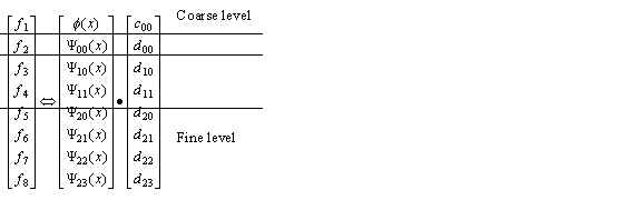
Forward and inverse wavelet transforms can be expressed shortly in terms of matrix
multiplication:
D = R-1*F (21)
F = R*D (22)
where R is reconstruction matrix and R-1 is decomposition matrix. Elements in R are values of the scaling function f(x) and wavelet basis functions Yjk(x), xОL.
For example, let F = (1, 0, -3, 2, 1, 0, 1, 2). The following matrix equation provides connection between F and
Haar wavelet coefficients. Haar wavelet basis is shown of fig.3.
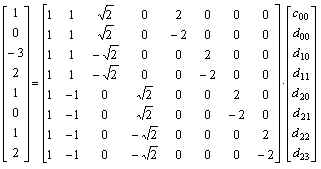
The solution is D = (1/2, -1/2, 1/2Ц2, -1/2Ц2,1/4, -5/4, ј, -1/4).
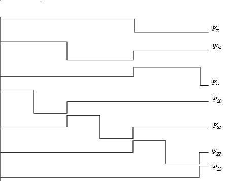
Fig.3. First 7 wavelets from Haar wavelet basis.
The idea behind wavelets is to analyze according to scale. In other words the purpose of
wavelet transform is to approximate function f at different scales (i.e.
analyzing either small or gross details). Based on fig.3. we can get the following
approximations of the function f:
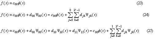
The more wavelet coefficients used to approximate the function the better is the approximation. Important thing is that each approximation (23)-(25) depicts details at different level of resolution.
It is helpful to think of coefficients ck as a filter. Coefficients are placed in transformation matrices H and G applied to the data vector F. H works as a smoothening filter (low-pass filter), and G works to bring out data's “detail” (high-pass filter). Matrices G and H form a quadrature mirror filter pair (QMF).
Wavelet transform is normally implemented on the base of Mallat's tree
algorithm or pyramidal algorithm [2]. Wavelet coefficient matrix is applied to the
data in hierarchical order. The wavelet coefficients are arranged so that odd rows contain
an ordering of wavelet coefficients that act as smoothening filter, and the even rows
contain an ordering of wavelet coefficients that act to bring data's detail. The matrix is
first applied to the original, full-length data vector. Then vector is smoothed and
decimated by half and the matrix applied again. Process continues until a trivial number
of data remain. That is, each matrix application brings out higher resolution of the data
while at the same time smoothening the remaining data. The output of discrete wavelet
transform (DWT) consists of the remaining “smooth” components, and all of the
accumulated “detail” components. The DWT matrix is not sparse in general. The same
approach as in FFT is used to boost computations - DWT matrix is factorized into a product
of a new sparse matrices. The result is the algorithm of Mallat and Daubechies that
requires only O(N) operations to transform N-sample vector, or O(Nlog2N)
operations until a trivial number of data remain.
3.2. Mallat's pyramidal algorithm
Mallat's pyramidal algorithm operates on finite set An of n=2N input data. Filters H and G applied to this data and create output streams that are half of the length of the original input.
Decomposition or forward wavelet transform can be described by the following equations:
Aj-1 = HAj (26)
Bj-1 = GAj, j = N,…1 (27)
Equation for reconstruction or inverse wavelet transform is
Aj = H*Aj-1 + G*Bj-1 (28)
Matrices H and G are defined by the following equations:
Hij =1/2 c2i-j (29)
Gij = (-1)j+1cj+1-2i (30)
Note filter matrices G and H have twice as much columns as rows. Forward wavelet transform starts with G and H of size n x 2n. At each step of transform calculated vector Aj-1 (and Bj-1) is twice as short as Aj (Bj). The number of columns and rows in G and H decreases by 2 with each step, until the limit of 1 x 2 reached and the last Aj-1= A0 and Bj-1= B0 produced, both containing only one element. Inverse wavelet transform reverses this process.
Transposed matrices G and H without Ѕ coefficient form dual filters G* and H*
H*ij = c2j-i (31)
G*ij = (-1)j+1ci+1-2j (32)
Partial matrices H and G are shown on fig.4.
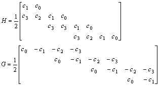
Fig.4. Partial matrices H and G.
Shown rows 1…4 and columns 1..8. By their construction filters H and G are orthogonal:
HG*=0 (33)
Also it can be shown that
LL* = 1 (34)
HH* = 1 (35)
L*L + H*H = 1 (36)
3.3. Pyramid algorithm implementation
Actually no matrix multiplication performed in
practice. Rather data values fi convolved with filter coefficients.
The output of low-pass filter (Hf)i is
![]()
The output of high-pass filter (Gf)i is
![]()
In many cases the odd, or low-pass filter has the most of the “information content” of the original input signal. The even, or high pass output contains the difference between the true input signal and the value of the reconstructed input if it were to be reconstructed only from the information given by the odd output. In general higher-order wavelets tend to put more information into the odd output and less into the even output. If the average amplitude of the even output is low enough, then the even half of the signal may be discarded without greatly affecting the quality of the reconstructed signal. An important step in wavelet-based data compression is finding wavelet functions, which causes the even terms to be nearly zero.
If the signal is reconstructed by inverse low-pass filter of the form
![]()
then the result is duplication of each entry from the low-pass filter output. The perfect reconstruction is a sum of the inverse low-pass and inverse high-pass filters and the perfectly reconstructed signal is
![]()
f = fL + fH (41)
Since most of the information exists in the low-pass filter output it
makes sense to take that filter output and transform it again, to get new two sets of data
each one quarter the size of the original input. Each step of transforming the low-pass
output is called a dilation and if the number of input samples n = 2N
then a maximum of N dilations can be performed, the last dilation resulting in a
single low-pass value and single high-pass value.
In wavelet decomposition the filter H is an “averaging filter” while its mirror counterpart G produces details. When wavelet coefficients corresponding to details are small they might be omitted without substantially affecting the original data. Thus the idea of thresholding wavelet coefficients is a way of cleaning out “unimportant” detail considered to be noise.
The policy for hard threshold is keep or kill. The absolute values of wavelet coefficients are compared to a fixed threshold l. If the magnitude of the coefficient is less then l, the coefficient is replaced by zero:
Soft thresholding shrinks all the coefficients towards the origin:
djk = sign(djk)(|djk| - l)+ (43)
A certain percent of smallest wavelet coefficients replaced with zeros.
Proposed by Donoho and Johnstone [3] universal threshold l on transformed data set yi/n, where n is the sample size, and s is the scale of the noise on a standard deviation scale. Universal thresholding can be used along with hard or soft thresholding methods.
![]()
4. Wavelet applications
Compression of digital images is brought to eliminate redundant information. There are three types of redundancy:
Spatial Redundancy. In almost all images, the values of neighboring pixels are strongly correlated.
Briefly speaking, compression is accomplished by applying a wavelet transform to decorrelate the image data, quantizing the resulting transform coefficients, and coding the quantized values [4]. Image reconstruction is accomplished by inverting the compression operations (fig.5.).
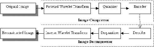
Fig.5. Block diagram of wavelet-based image compression / decompression.
The forward and inverse wavelet transforms can each be efficiently implemented in O(n) time by a pair of appropriately designed quadrature mirror filters. The one-dimensional forward wavelet transform of a signal s is performed by convolving s with both H and G and downsampling by 2. The relationship of the H and G filter coefficients with the beginning and ending of signal is shown on fig.6.
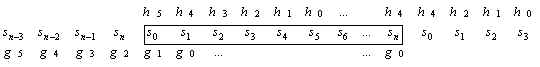
Fig.6. Relationship of the filter coefficients with the signal endpoints.
Note G filter extends before the signal in time and H filter extends beyond the end of the signal. A similar situation is encountered with the inverse wavelet transform filters H* and G*. Suitable padding values can be produced with the signal wrapped about its endpoints. Block diagram of the 2-D wavelet forward and inverse transforms shown on fig.7. and fig.8. respectively.
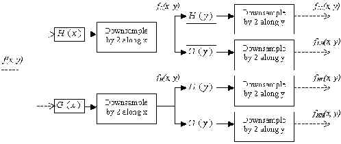
Fig.7. Block diagram of the 2-D forward wavelet transform.
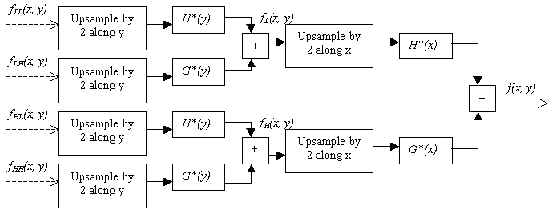
Fig.8. Block diagram of the 2-D inverse wavelet transform.
The image f(x, y) is first integrated along the x dimension, resulting in a
low-pass image fL(x, y) and a high-pass image fH(x, y).
Since the bandwidth of fL and fH along the x
dimension is now half that of f, we can safely downsample each of the filtered
images in the x dimension by 2 without loss of information. The downsampling is
accomplished by dropping every other filtered value. Both fL and fH
are then filtered along the y dimension, resulting in four subimages: fLL ,
fLH, fHL , and fHH , and downsample. 2D
filtering decomposes an image into an average signal fLL and three
detail signals which are directionally sensitive: fLH emphasizes the
horizontal image features, fHL the vertical features, and fHH
the diagonal features.
Averaged signal fLL can be transformed recursively once again. The
number of transformations performed depends the amount of compression desired, the size of
the original image, and the length of the QMF filters. In general, the higher the desired
compression ratio, the more times the transform is performed.
After the forward wavelet transform is completed, we are left with a matrix of
coefficients that comprise the average signal and the detail signals of each scale, and no
compression of the original image has been accomplished yet. Compression is achieved by
quantizing and encoding the wavelet coefficients.
The forward wavelet transform concentrates the image information into a relatively small
number of coefficients. The elimination of small valued coefficients can be accomplished
by applying a thresholding function to the coefficient matrix (see 3.4.). The amount of
compression obtained can now be controlled by varying the threshold parameter l.
Higher compression ratios can be obtained by quantizing the nonzero wavelet coefficients
prior to encoding. Best results achieved when a separate quantizer designed for each
scale.
Fig.9. Reconstructed images for wavelet and JPEG image compressors.
Experiments with wavelet-based image compression show that at compression ratios above
30:1, JPEG performance rapidly deteriorates, while wavelet coders degrade gracefully well
beyond ratios of 100:1 (fig.9).
Daubechies W6 wavelet is used for the wavelet transform. Compression ratio is
64:1.
4.2. Video Compression
The wavelet transform can also be used in the compression of image sequences, or video.
Video compression techniques are able to achieve high quality image reconstruction at low
bit rates by exploiting the temporal redundancies present in an image sequence. The
computational expense of the wavelet transform implies the use of high-speed CPUs or
accelerator hardware.
However the amount of computations can be significantly
reduced by running inverse wavelet transform only on pixels presenting difference ![]() fi between two adjacent frames fi
and fi+1, i.e. eliminating redundant firstorder temporal
information.
fi between two adjacent frames fi
and fi+1, i.e. eliminating redundant firstorder temporal
information.
Simple video codec using wavelet transform is shown on
fig.10.
There is spatial redundancy in Dfi , and this redundancy can be reduced by
application of some wavelet transform W. Thresholding can now be performed on the
transformed difference image W(![]() fi)
to eliminate image changes that are considered too small to be meaningful. After
thresholding, we have an approximate transformed difference image W(
fi)
to eliminate image changes that are considered too small to be meaningful. After
thresholding, we have an approximate transformed difference image W(![]() fi) that is extremely sparse. W(
fi) that is extremely sparse. W(![]() fi) is then analyzed to determine
which portions of the inverse wavelet transform will need to be performed to reconstruct
an approximation
fi) is then analyzed to determine
which portions of the inverse wavelet transform will need to be performed to reconstruct
an approximation ![]() fi of
the i-th difference image. This information is then encoded and sent to the video
decoder.
fi of
the i-th difference image. This information is then encoded and sent to the video
decoder.
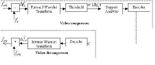
Figure 10: Block diagram of the wavelet-based video codec.
Using the information sent by the encoder, the decoder can reconstruct ![]() fi . Because of its sparse
nature,
fi . Because of its sparse
nature, ![]() fi can be
reconstructed very quickly by computing the inverse wavelet transform for only those
pixels influenced by the coefficients sent by the encoder. We assume that the decoder has
available some approximation fi of frame i, so the next frame
in the sequence can be constructed as
fi can be
reconstructed very quickly by computing the inverse wavelet transform for only those
pixels influenced by the coefficients sent by the encoder. We assume that the decoder has
available some approximation fi of frame i, so the next frame
in the sequence can be constructed as
![]()
Developments in the field of artificial vision for robots appear to be natural wavelet applications. In order to build reliable artificial vision algorithms the following fundamental questions have to be answered:
David's Marr (MIT Artificial Intelligence Laboratory) theory states that
intensity changes occur at different scales in an image, so that their optimal detection
requires operators of different sizes. Also abrupt intensity changes produce peaks or pits
in the first derivative of the image. These two statements require that a vision filter
have two characteristics: it should be a differential operator, and it should be capable
of operating on desired scale. New type of wavelet was developed called “Marr wavelet”
to address this problem.
Various applications dealing with incomplete or noisy data require “true” signal recovery. It could be geology and seismic wave study, image processing, sound processing, spectroscopy etc. Wavelet shrinkage and thresholding method was developed to address this problem [5].
This technique works the following way. Data is decomposed using wavelets. Two types of filters are used: averaging and the one detail ones that produce details. Wavelet coefficients corresponding to minor details (i.e. less then particular threshold) can be discarded and replaced with zeros without seriously affecting data accuracy. These coefficients is used in inverse wavelet transform to reconstruct the data. The main advantage of wavelet-based denoising is that smoothening of the data was achieved without loosing “sharp” features (fig.11.).
Denoising algorithm developed by David Donoho consists of the following steps:
1. Transform the image into wavelet coefficients using Coiflets with three vanishing moments;
2. Apply threshold at two standard deviations.
3. Perform inverse wavelet transformation to reconstruct the image.
Fig.11. Original and denoised Nuclear Magnetic Resonance signal.
Wavelet packets (linear combination of wavelets) can be very useful in sound synthesis [6]. Main idea is that a single wavelet packet generator could replace a large number of oscillators. Sound of a particular instrument can be decomposed into wavelet packet coefficients. Reproducing a note would then require inverse wavelet transformation and application of envelope generators to the final waveform.
There are two main advantages of wavelet packet based music synthesizer:
wavelet packet coefficients, like wavelet coefficients are quite small for smooth signals (and most sound are smooth);
Wavelet analysis appears to be a very powerful tool for characterizing self-similar behavior over a wide range of time scales.
In 1993 quasi-periodic oscillations (QPOs) and very low frequency noise (VLFN) from an astronomical X-ray accretion source, Sco X1 were investigated at NASAAmes Research Center [7]. Sco X1 is a member of a close binary star system with a compact star generating intense X-rays.
The researchers noticed that the luminosity of Sco X1 varied in a selfsimilar manner, that is, the statistical character of the luminosities examined at different time resolutions remained the same. Since one of the great strengths of wavelets is that they can process information effectively at different scales, new wavelet tool called a scalegram was used to investigate the timeseries.
A scalegram of a time series as the average of the squares of the wavelet coefficients at a given scale. Plotted as a function of scale, it depicts much of the same information as does the Fourier power spectrum plotted as a function of frequency.
The scalegram for the timeseries clearly showed the QPOs and the VLFNs, and subsequent simulations suggested that the cause of ScoX1's luminosity fluctuations might be due to a chaotic accretion flow.
Ultrasound imaging can benefit as well from the use of wavelets. Basic
goal is to get superior image quality while retaining important image details. Generally
raw data images produced by ultrasound devices contain substantial deal of noise and look
blurry. Certain physical phenomenons and limitations imposed by nature control the quality
of ultrasound image.
Ultrasound transducers produce sound pulses of certain frequency (2 - 50MHz) which travel
through the object being investigated. Reflected echo-signals are recorded and form
A-scan. B-scan or in other words raster image can be produced combining A-scans
corresponding to different spatial locations in the object.
In general it is desired to have high frequency transducer such that resolution of smaller
details will be possible. On the other hand high frequency ultrasound decays faster and as
a result reflections are weaker. For most medical applications 2 - 3.5MHz transducers are
used. Moreover ultrasound transducers produce pulse consisting of several decaying wiggles
which give raw data image its blurry appearance. Some noise produced due to multiple
reflections and sound scattering. These effects are normally small in medical
applications.
There are two distinct areas of wavelet application in ultrasound imaging.
The latter technique employs generation of wavelet-like pulses by ultrasound transducer.
Ideally L-wavelet pulses (translated square wave) or their close approximation must be transmitted:
![]()
In this case reflected echo signal will present combination of dilations
and translations of the same mother wavelet (L-wavelet). Fast wavelet transform performed
on A-scan data yields wavelet coefficients corresponding to the value of acoustic
impedance at different depth.
Fig.12. Ultrasound reflected signal and wavelet transformation reconstructed image
The image on the left is the calculated ultrasound signal taken in a plane
through the center of a tomato. The image on the right is the result of performing wavelet
transformation reconstruction algorithm.
Wavelet theory is highly developed field of mathematics and it's being constantly refined. Refinement involves generalizations and extensions of wavelets resulting in yet even more exciting wavelet packets technique.
Current researches involve development of wavelet applications, such as data analysis (astrophysics, seismology, statistics), still image and video sequence compression, sound generation, operator analysis, noise filtering, ultrasound imaging and yet more to come.
Constant growth of computational power opens new possibilities for the use of wavelets, making possible implementation of video compression at compression ratios near 1000:1 and almost 100:1 for still image.
Examples of recent wavelet applications are fingerprint image compression used by FBI [9] and digital filtering for evolving standard of High Definition Television (HDTV). Hardware wavelet transformer chips geared towards DSP applications were designed and implemented [10].
Despite of their nice properties wavelets won't replace traditional
Fourier transform and its modifications (such as Windowed Fourier Transform) everywhere.
Wavelets are likely to prevail in applications dealing with abruptly changing signals and
signals with discontinuities. And even more interesting wavelet applications lay in the
uncharted territory of the future.
References
1. I.Daubechies, Orthonormal Basis of Compactly Supported Wavelets, Comm. Pure Applied Mathematics, vol.41, 1988, pp.909-996.
2. S.Mallat, A Theory of Multiresolution Signal Decomposition: The Wavelet Representation, IEEE Trans. Pattern Analysis and machine Intelligence, vol.11, 1989, pp.429-457.
3. D.Donoho, I.Johnstone, G.Kerkyacharian, D.Picard, Density Estimation by Wavelet Thresholding, Technical Report, Department of Statistics, Stanford University
4. M.Hilton, B.Jawerth, A.Sengupta, Compressing Still and Moving Images with Wavelets, Multimedia Systems, Vol.2, No. 5, 1994, pp.218-227.
5. D.Donoho, “Nonlinear Wavelet Methods for Recovery of Signals, Densities, and Spectra from Indirect and Noisy Data”, Different Perspectives on Wavelets, Proceeding on Symposia in Applied Mathematics, Vol. 47, I., Daubechies ed. Amer. Math. Soc., Providence, R.I.,1993, pp.173-205.
6. V.Wickerhauser, Acoustic Signal Compression with Wave Packets, 1989, available by anonymous FTP at pascal.math.yale.edu, filename: acoustic.tex.
7. J.Scargle, The QuasiPeriodic Oscillations and Very Low Frequency Noise of Scorpius X1 as Transient Chaos: A Dripping Handrail?, Astrophysical Journal, Vol. 411, 1993, L91L94.
8. J.Letcher, An Imaging Device that Uses Wavelet Transformation as the Image Reconstruction Algorithm”, International Journal of Imaging Systems and technology, Vol. 4, 1992, pp.98-108.
9. T.Edwards, Discrete Wavelet Transforms: Theory and Implementation, 1992.
10. J.Bradley, C.Brislawn, T. Hopper, The FBI Wavelet / Scalar Quantization Standard for Gray-scale Fingerprint Image Compression, Tech. Report LA-UR-93-1659, Los Alamos National Lab, Los Alamos, N.M. 1993.
Tulsa, USA
Поступила в редакцию 12.12.1998.